
Your Trial Is Not Behind Schedule. It Is in the Wrong Place.
The geometrical principles of operational failure in clinical development

There is a particular kind of meeting that happens in clinical development about fourteen months into a Phase 3 trial. The enrollment forecast was revised twice. The site rescue program has been running for three months. A third revision is being drafted. The task force — originally assembled to identify underperforming sites and fix them — has stopped asking why the sites are behind and has started negotiating how much the timeline needs to move.
Nobody in the room is incompetent. The sites are not badly run. The CRO is not negligent. The data management team is not behind. And yet the trial is in trouble — structurally, irreversibly, in a way that more site visits and more patient recruitment support will not fix.
The reason is geometric. The trial entered its execution phase with operational assumptions that were sitting near a mathematical boundary — a threshold below which normal variation in execution is absorbed, and above which small additional degradations produce a catastrophic, irreversible cascade. Nobody identified that boundary before the trial started. Nobody monitored the distance to it during execution. By the time the meeting happens, the program crossed it six months ago.
This essay is about that boundary. What it is, how to find it before it finds you, and what operational management looks like when you take it seriously.
Part One: Three ideas in plain English
Fractals: why the same problem exists at every level
A fractal is a system where zooming in reveals the same pattern you saw when zoomed out. The canonical image is a tree: the trunk splits into major branches, each branch splits into smaller branches, each smaller branch splits into twigs, each twig ends in something that looks like a tiny tree. The structure repeats perfectly at every scale.
A clinical trial is also a fractal. The operational hierarchy — Program, Region, Country, Site, Patient — has the same structure at every level. And more to the point, the same set of operational problems appears at every level: activation delays, resourcing gaps, vendor dependencies, compliance risk, and communication lag. The pattern repeats.
This has one specific and uncomfortable implication. In a fractal system, a failure at an upper level does not produce one problem. It produces N problems simultaneously, where N is the number of nodes below it. A protocol amendment at the program level does not change one thing. It touches every region, every country, every site, and every patient currently in the trial — simultaneously. The amendments arrive at different teams at different times and appear unrelated. They are not. They share a common origin.
Why this matters operationally
When multiple sites show the same failure pattern simultaneously, the correct question is not ‘what is wrong with these sites?’ It is ‘what upstream node failure is generating this pattern across the network?’ The answer changes both the intervention and the urgency.
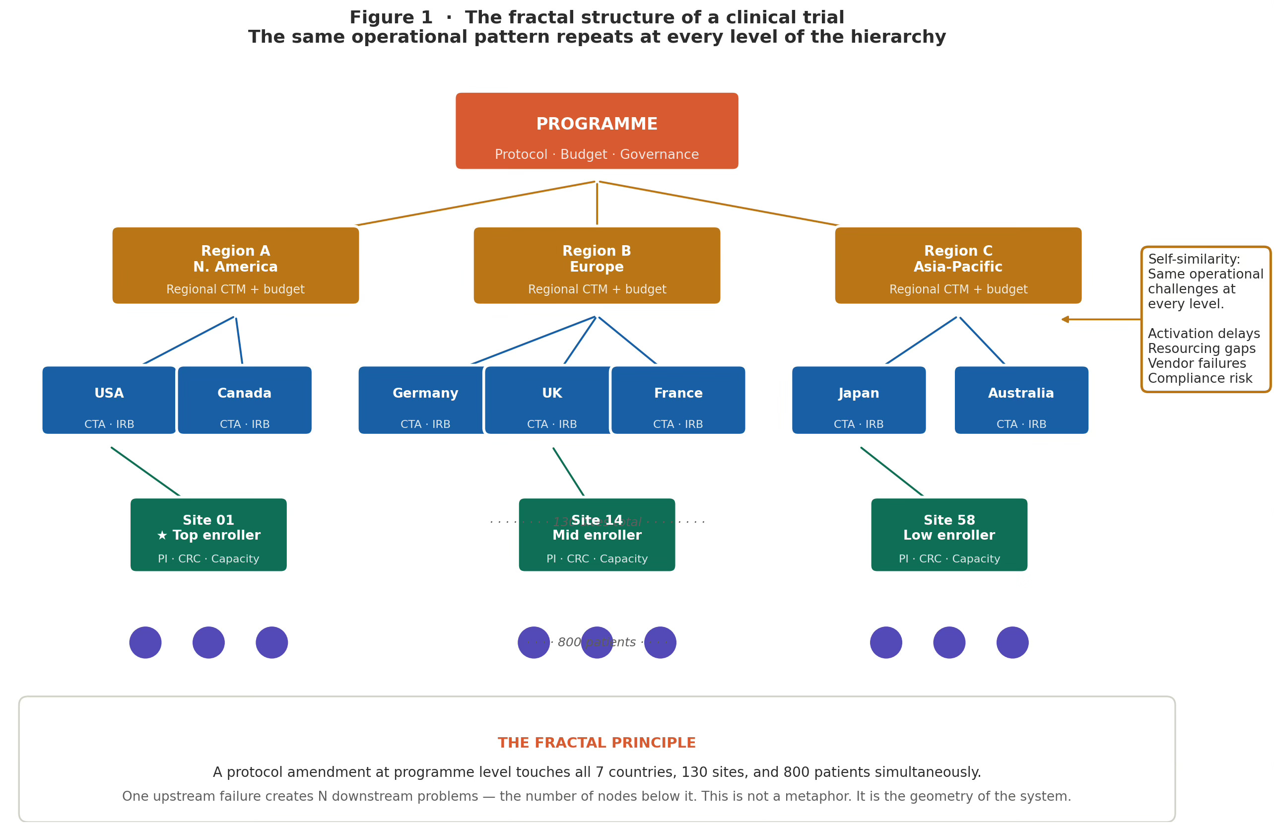
Figure 1 · Fractal Structure of a Clinical Trial
The fractal structure of a clinical trial. Program → Region → Country → Site → Patient. The same operational challenges repeat at every level. A disruption at the program level creates N simultaneous downstream problems — one per node below it. Self-similarity means a regional-level signal is a leading indicator of site-level failures that have not yet surfaced.
The Mandelbrot set: the map of operational stability
The Mandelbrot set is, in essence, a map of all possible starting configurations — showing which ones produce stable, bounded outcomes and which ones spiral out of control. The boundary between the two zones is the mathematically interesting part: it is infinitely complex, and a single step on either side determines everything.
You do not need mathematics to use this idea. Every clinical trial has a composite set of operational assumptions: site activation pace, screen failure projections, CRO capacity estimates, country regulatory timelines, dropout assumptions, IP shelf-life relative to the enrollment window. Think of this composite as a single point on a map. The Mandelbrot set tells you whether that point is in the stable zone (where normal execution variance is absorbed and the trial delivers), near the boundary (where modest degradation in any single parameter flips the trial to unrecoverable), or in the escaped zone (where no operational excellence can fix the structural incompatibility between the protocol and the execution plan).
The practical observation is this: most programs that enter execution in trouble are not in the escaped zone. Their operational plan was not fundamentally broken. It was near the boundary — sitting in a region where a screen failure rate drifting from 2:1 to 3:1, combined with a single key country running two regulatory cycles behind, combined with a modest CRO staffing reduction, was sufficient to push the composite past the threshold. None of those three events triggered an alarm individually. Together, they crossed the boundary.
The question of feasibility never asks
Standard feasibility asks: are our site and enrollment assumptions reasonable? The right question is: how much degradation across our assumptions is needed to make the trial unrecoverable — and are we comfortable with that margin? A parameter can pass every reasonableness check and still be sitting at the operational boundary.
Figure 2 · The Mandelbrot Set – operational parameter space
The Mandelbrot set as an operational stability map. Each pixel = one combination of operational parameters. Dark interior: orbit stays bounded — trial is robust. Colored boundary zone: orbit escapes slowly — trial is near its operational fragmentation threshold. Most operational failures originate here. Marker A (stable), B (boundary), C (escaped) illustrate three program positions.
Julia sets: how sensitive is your trial to starting conditions?
For each specific operational configuration — each position on the Mandelbrot map — there is a corresponding Julia set: a picture of which starting conditions (which sites activate first, which patients enrol early, which country comes online when) lead to trial success and which lead to failure.
When the operational composite is well within the stable zone, the Julia set is a single connected region. A wide range of starting conditions all lead to the same place: trial success. Whether Site 01 activates first or Site 58, whether Germany comes online in month 3 or month 7, the trial delivers. The outcome is robust to execution sequence.
When the composite is near the Mandelbrot boundary, the Julia set fractures into a lacy, thread-thin structure riddled with gaps. Now it matters intensely which sites activate first. If the high-enrolling sites happen to activate late and the low-enrolling sites fill the early cohort, the program enters a recovery trajectory it cannot complete within the timeline — even with full rescue operations. The same protocol, the same sites, a different activation sequence: different outcome. This is not bad luck. It is the structural property of a fragmented Julia set.
When the composite is outside the boundary, the Julia set fragments into disconnected dust. There is no connected basin of successful starting conditions. Some windows may briefly enrol adequately. The overall system cannot sustain itself.
The clinical translation
When a Phase 2 program produces the result ‘it worked in one subgroup analysis but not the overall population,’ the team typically looks for an operational explanation. Often, there is no satisfying one. The more accurate explanation is geometric: the program was running in the fragmented zone of its Julia set. Different patient cohorts were enrolled in different sequences, ending up in different disconnected regions of the outcome space. This is not noise. It is structure.
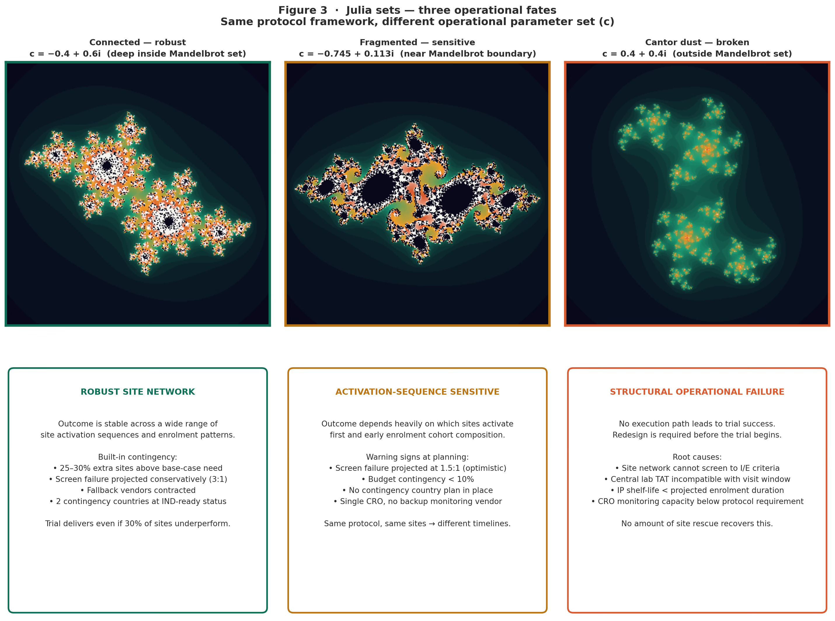
Figure 3 · Julia sets –– 3 operational fates
Julia sets — three operational fates. Left (connected): robust site network, wide basin of successful starting conditions. Center (fragmented): outcome highly sensitive to site activation sequence — same protocol, different timeline depending on which sites activate first. Right (Cantor dust): structural operational failure — no execution path leads to success.
Part Two: What to actually do
The framework generates four specific operational responses, each timed to a distinct phase of program management.
Stage 1 — Diagnose: map the parameter composite before the trial starts
The diagnosis happens at operational planning, before the first CTA submission. For each high-branching operational parameter — the ones whose failure cascades to multiple levels simultaneously — calculate two numbers: the current planned value, and the value at which the failure becomes irreversible. The distance between them is what matters.
This is not a standard risk register. Risk registers list risks and their probabilities. A parameter distance analysis maps how far each assumption sits from its fragmentation threshold. A parameter can have a low probability of failure and still be near the boundary — if the threshold is close to the planned value, normal variation is enough to cross it.
The parameter distance table
For each high-branching parameter:
• What is the planned value?
• What is the failure threshold — the value at which the cascade becomes irreversible?
• What is the distance between them?
• What is the typical variance for this parameter in comparable programs?
• Is the variance larger or smaller than the distance?
Parameters where the typical variance is roughly equal to the distance — or greater — are Amber-zone parameters. They need structural mitigation before the trial begins. Parameters with large distance-to-variance ratios are in the stable interior. Standard monitoring is sufficient.
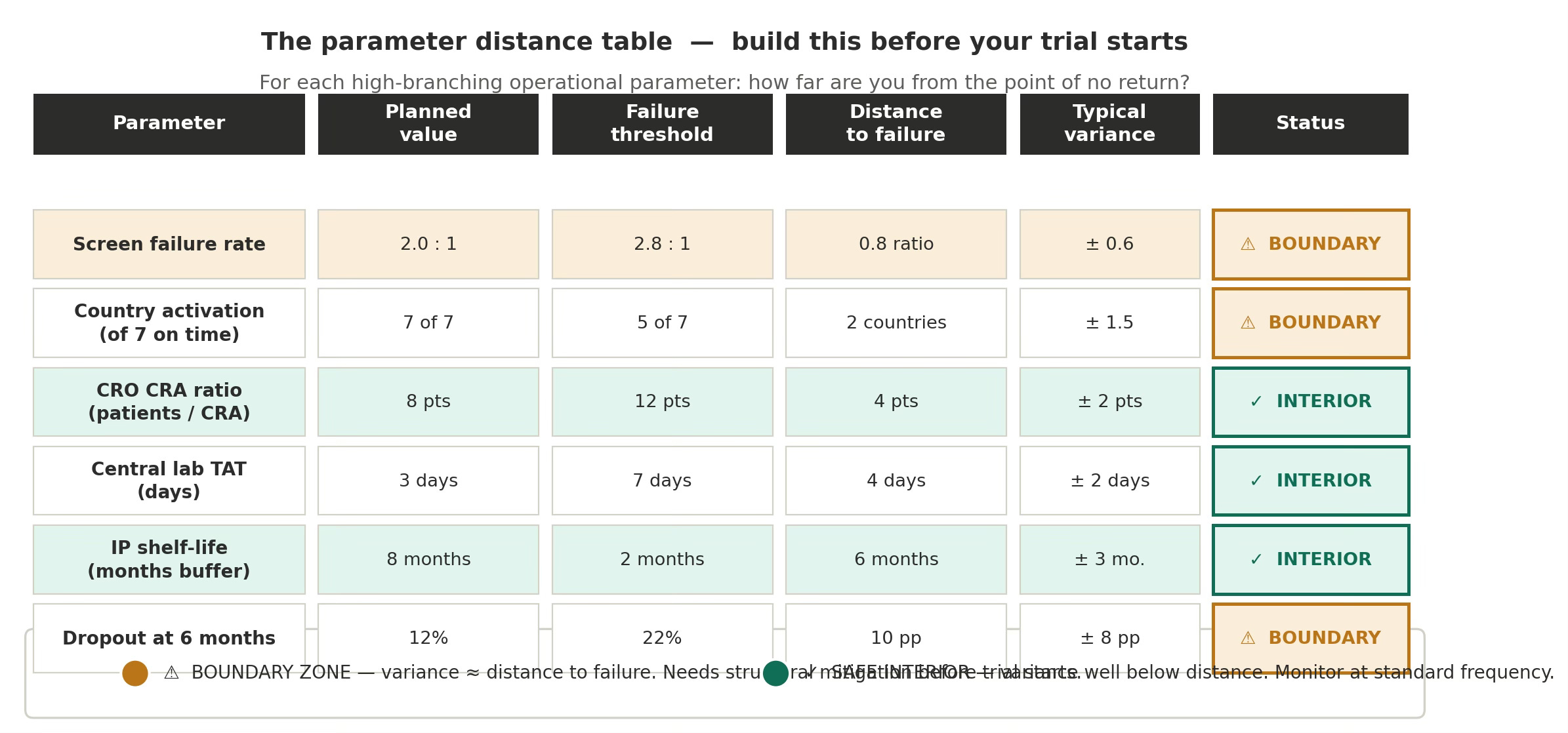
Figure 4 · Paramater distance
The parameter distance table — the practical instrument. Six named Phase 3 parameters with planned value, failure threshold, distance, and variance. Screen failure rate and country activation are Amber-zone: typical variance is within the range of the distance to failure. These require structural mitigation at the design stage, not monitoring improvements.
Stage 2 — Prevent: build structural margin into boundary-zone parameters
Prevention happens at protocol design and vendor contracting. For each Amber-zone parameter, the response is structural — not a monitoring improvement, but a design change that increases the distance to the fragmentation threshold.
Screen failure rate
If screen failure is an Amber parameter, the response is over-siting: activate 25–30% more sites than the base-case model requires, specifically targeting sites with documented high-volume screening capacity in this indication. The cost is higher activation spend. The cost of not doing it is a mid-trial boundary crossing with no recovery path.
Country activation
If country activation is Amber, the response is country redundancy: identify two additional countries that can be added within 90 days if any primary country misses its critical activation milestone. These contingency countries should be at IND-ready status before primary country submissions begin. This is deliberate Julia set engineering — expanding the connected basin of viable execution outcomes so that a wider range of country activation sequences all lead to on-time enrollment.
Vendor capacity
If CRO monitoring capacity is Amber, the contractual response is a minimum staffing clause with a financial penalty for falling below the committed CRA-to-patient ratio, plus a pre-negotiated right to bring in a backup CRO within 60 days if the clause is triggered. This keeps the parameter in the stable interior even if the primary vendor experiences staffing disruption.
Stage 3 — Mitigate: classify before you intervene
When operational problems surface in a running trial, the first question is classification, not intervention. Is this a leaf failure or a branch failure?
• A leaf failure is localized to a specific node — one site, one country, one vendor interaction. It has limited downstream spread. Local intervention works.
• A branch failure has its origin at a high-branching node, and produces the same class of problem at multiple leaf nodes simultaneously. Local intervention does not work because the cascade from the upstream node continues arriving at new leaves faster than you can remediate existing ones.
The diagnostic test is structural: do the failing nodes share a common upstream cause? Seven geographically dispersed sites, all reporting high screen failure rates in the same two-month window, are not seven simultaneous leaf failures. It is one branch failure — the inclusion criteria are eliminating the available patient population, manifesting at seven leaves at once.
Once a branch failure is classified, the intervention moves up the hierarchy: protocol amendment, inclusion-criterion modification, CRO contract action, or country portfolio change. This requires more organizational authority and faster escalation than a leaf intervention. The fractal framework argues for keeping that escalation path short and pre-rehearsed, because branch failures require decisions at exactly the moment when organizational pressure is highest to continue with incremental leaf-level rescue.
Pre-committed branch-level triggers
For each Amber-zone parameter identified at Stage 1, specify in advance: the trigger threshold, the response, and the response time. For example, if screen failure exceeds 2.5:1 for two consecutive months, activate contingency sites and convene an I/E review within 30 days. Pre-commitment removes the decision from the moment of maximum pressure to continue.
Stage 4 — Monitor: track distance, not just performance
Standard operational monitoring tracks performance against target: enrollment curve, data completeness, protocol deviation rates, and site performance rankings. These are all leaf-level outputs. They show what has already happened at the leaves.
Parameter distance monitoring tracks the operational composite against its fragmentation thresholds — at the branch level, at sufficient frequency to detect boundary drift before it manifests at the leaves.
The living parameter map
The parameter distance table from Stage 1 becomes a living document, updated monthly for Amber-zone parameters and quarterly for stable-interior parameters. For each parameter, track: current value, trend direction, distance to threshold, and rate of boundary approach. A parameter performing within target but drifting toward its threshold is a leading indicator — it requires attention before it becomes a problem.
Branch-level leading indicators
Because the trial hierarchy is self-similar, a regional-level anomaly is a leading indicator of site-level problems that have yet to surface. A regional screen failure rate running 20% above the trial average is not yet a crisis — individual sites in that region may each be within normal variance. But the regional branch signal indicates that leaf-level failures are imminent. The structure of the system commits them before they appear.
Acting on the regional signal rather than waiting for individual site flags is the difference between early-stage intervention and late-stage rescue. In a program near the Amber boundary, it is sometimes the difference between a recoverable adjustment and an unrecoverable cascade.
The underlying principle
All four stages of this framework rest on one observation that fractal mathematics makes precise:
In complex, branching, self-similar systems — which is what a Phase 3 clinical trial is — the information that predicts failure is structurally available before the failure occurs. It sits at the branch level, weeks to months before it is visible at the leaf level.
The operational task is never ‘what went wrong?’ It is always ‘what branch failure is generating the leaf signals we are currently seeing, and how long ago did it occur?’
The failure rate in Phases 2 and 3 is not primarily a failure of science or execution. It is a failure of parameter awareness — of not knowing, at the moment when it would be actionable, how close the program’s operational assumptions are to the threshold where normal variation is sufficient to produce an irreversible cascade.
The Mandelbrot boundary does not care whether the assumptions were reasonable. It only cares whether the composite lies to its right. Knowing where the boundary is — before the trial starts — is the whole job.
The companion LinkedIn post (Biotech Triallist newsletter) covers the practical tools without the framework — parameter distance table, three-zone classification, and the leaf-vs-branch diagnostic. The figures referenced throughout this piece are available as downloadable PNG files.